Home Science Page Data Stream Momentum Directionals Root Beings The Experiment
Let us examine this D Series, upon which so much is based, a little more closely.
What have we established? In the first section we looked at another representation of numbers, the infinite continued fraction. We saw that it was a precise way of representing all rational square roots, hence all integers. This was a way of putting rational numbers and square roots in the same family. In order to evaluate these infinite continued fractions, we broke them into the Infinite Continued Fraction Series, the F Series. Each member of the series was a finite approximation of the infinite continued fraction. The infinite member of the set was the infinite continued fraction. Further it was seen that the members of the Fraction Series were actually a ratio of consecutive members of a series called the Denominator Series. It was seen that these infinite continued fractions could be written as a limit of the ratio of consecutive members of the D Series.
Below is the standard Denominator Series for Square Roots, written in alternate style, where d(N-R) = D(R).
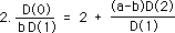
Dividing through by b D(1).
Subtracting 1 from each side of the equation.
This is just a simple way to get to this common expression that should be familiar from the previous section.
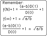
As N becomes larger and larger, the limits of these ratios of the D Series approach the square root of our rational number, a/b.
This is where we started our exploration.
This sequence just shows that the relation between the F Series and its inverse, the F’ Series, can be derived directly from the D Series. Although we derived our D Series from the F Series the D Series is foundational to the F Series, just like atoms are at the foundation of molecules. The F Series, which is based upon the infinite continued fractions used to generate the square roots of all positive rational numbers, is generated from the ratio of the members of the D Series.
Another interesting feature of the D Series was that the Pattern of the series was more important than the seed, i.e. the initial point of the series. The Limit of the D Series is independent of starting point, i.e. ‘seeds’, especially in the center. The Pattern of the D Series dominates any numbers, or seeds, that were used to get the series going. No matter which values were used the Pattern of the D Series drove the ratio towards the Limit. With the D Series, Pattern dominates Number.
As seen the D Series has many interesting properties. Now we will explore its Geometric Nature by analyzing the ratio between its elements.
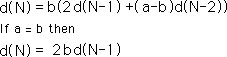
A special feature of the D Series for square roots is that it requires the two previous elements of the series to generate the present element. Below is a discussion of a special case of the D Series, which only requires the immediately preceding element to generate the next. We start with the general D Series.
When a = b, the N-2 term drops out in the D Series. This leaves us with the basic geometric series. Multiply each term by 2b to get the next term in the series. If b is one and d(1) =1, then our series becomes the familiar, 1, 2, 4, 8, 16, 32, 64,128, …. If we allow b to be any real number then we can generate any geometric series.
What happens to our F Series when a = b? If a = b, √a/b always equals one. Remember that the Limit of the F Series is the Root minus one. In this case the Root, √a/b , equals one. Consequently the Limit of the F Series is zero. Following is the algebraic expression: ƒ(∞) = √a/b - 1 = 1 - 1 = 0. This is the empty F Series, which just equals zero. There really is no Series, just zero. When the Root and Root Number are both one, then there is no series except the empty F Series, when all the members are zero.
While the F Series is empty, there are an infinite number of D Series Patterns, which are geometric. This exhibits the point that there are an infinite number of D Series Patterns which correspond with each F Series, just as there are an infinite number of fractions corresponding with each decimal. Remember that each fraction has an F Series that corresponds to it, from Theorem 1. Hence the set of all D Series is larger than the set of rational numbers. For each rational number there are an infinite number of D Series that will generate the same square root. 1/1, 3/3, 6/6 all equal one but each generate a different D Series. So the set of Denominator Series Patterns is infinitely larger than the set of rational numbers under the difference criteria introduced in another paper. The number of F Series is identical to the number of rational numbers.
We have seen that this special D Series, i.e. when a=b, is geometric. What about the general D Series? In this exploration, for simplification we will use the '≈' symbol to represent the limit as N approaches ∞. As an aside, we will mention that these limits are reached very quickly for numbers under 10 and very slowly for numbers over 100. We will see why when we look at these infinite ratios.
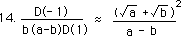
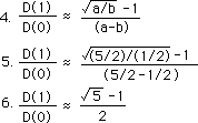
Looking at Equation 3 above and its limit in equation 5, we get the following approximation.
Multiplying through by D(1) and simplifying leads to this relation.
Multiplying the radical by b, we get,
This is the approximate ratio between consecutive members of the D series. This has been confirmed experimentally. See appendix.
Reversing the relationship we get this expression.
Simplified it becomes.
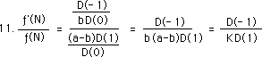
The ratio of the finite expressions, ƒ'(N) to ƒ(N), can be rewritten as follows. The D(0) terms drop out. Notice the emergence of our scaling factor, K = b(a-b), in the denominator.
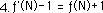
Below we write ƒ(N) as a function of ƒ'(N).
From previous results, we remember that x'/x = d, which is shown in another form below.
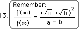
The limit of the ratio is given in equation 13. The finite ratio approximately equals the infinite ratio. Or the limit of the finite ratio as N approaches ∞ equals the infinite ratio, same difference.
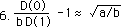
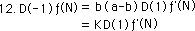
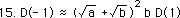
Solving for D(-1), we get.
Simplifying the coefficient of D(1) we get.
The ratio of D(-1) to D(1) approaches the square of the ratio between D(0) to D(1). This has also been confirmed experimentally. See appendix.
In a similar fashion the ratio between any two elements of our D series approaches the basic ratio between two consecutive elements raised to the power of the difference between the elements. This is expressed below. This too has been confirmed experimentally for a random number of samples.
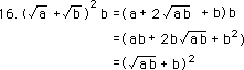
This sequence illustrates the geometric nature of the D Series. Each member is multiplied by a constant, √ab + b, to get the next member of the series. Apparently this second level iterative equation with all its internal structure reduces to a geometric series. Almost, not quite. These ratios are all approximate. Just as the above relation approximates the D Series, so does our perception of Reality approximate it.
There are a few differences between the geometric ratios for special D Series, when a=b, and the general D Series. The general geometric ratio of the D Series, shown above, is based upon square roots, while the geometric ratio of the special D Series is based upon exact integers. Second the ratio of the generalized series is approximate while the geometric ratio of the specialized D Series is exact. While there are differences it is easily seen that when a=b, as in this special case, that the general ratio becomes the special. It equals 2b our special case geometric ratio, √a√b+ b = √b√b + b = b + b = 2b.
The overall point of this section is to show that the D Series for square roots imitates a geometric series with √ab + b as its multiplier. Perhaps that should be restated to say that one way we can attempt to understand the D Series is to think of it as a geometric series. Just as electrons are not really little planets orbiting around a nucleus, neither is the D Series really a geometric series except in the special case when a=b. Indeed the geometric series only approximates the D Series, just as our perceptions only approximate reality. Although the geometric nature of the D Series is only a distorted reflection, it is a pretty good one. Most of our ratios are pretty close to the prediction. Further our 100% correlation indicates what a strong geometric linear relation exists. Let it be stressed that this relation could have been arithmetically linear, non-linear, or erratic without order. The highly ordered seemingly geometric nature of this relation while only approximating the reality of the D series is striking nevertheless. Similarly although a theory that closely fits the facts is intoxicating, one must always remember that the theory is still only a gross approximation of the Truth that lies behind.
We’ve been speaking of the D series as a 2nd order iterative equation, which means that it has two layers of feedback. There is a famous series that also has two layers of feedback, This is called the Fibonacci Series after its discoverer.
The Fibonacci series is based upon the sum of its two previous members. With our notation, it would be written as follows:
d(N) = d(N-1) + d(N-2).
This is the Fibonacci series. In form it looks very similar to our Denominator Series, which is also a function of the sum of its two previous members:
d(N) = 2b *d(N-1) + b(a-b)*d(N-2)
Is the Fibonacci sequence a special case of the D Series or something different? While the D Series has special coefficients for its past members, the coefficients of the Fibonacci series would just be one each. Can we fit this into the D Series framework?
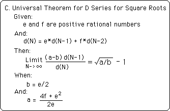
Let us solve for the general case, when the coefficients for the past elements are any rational numbers, e & f. Let us restate the problem in general terms. We know that the ratio of consecutive members of the D series leads to distinct and namable square roots. Do all second order iterative equations of this variety produce a namable Limit? Or stated another way, Are there any coefficients of the D Series that don’t lead to a square root?
Equation 1 is the general form of a second order iterative equation in the D Series format. For simplification we have let D(R) = d(N-R). Each new element of the series is formed by the sum of the two previous elements, each multiplied by a rational constant, e & f, shown in the equation below.
We don’t know much about the above equation. But we do know quite a bit about the equation below, which is the expression from the Denominator Series Theorem, which defines the D Series and its properties, including its connections to square roots.
For Eq. 1 to fit into the mold of Eq. 2, the coefficients of both equations must correspond. Therefore the ‘e’ of Eq. 1 must equal the ‘2b’ of Eq. 2. This is shown in Eq. 3. Dividing through by 2, we get equation 4, which shows b as a function of e.
Furthermore the coefficients of D(2) in Eqs. 1 & 2 must correspond. This equivalence is shown in Eq. 5.
In Eq. 6, we substitute the function of ‘e’ for b from Eq. 4 into Eq. 5. This leads to Eq. 6.
Switching the equation sides and dividing both sides by 2/e, we get Eq. 7.
Subtracting e/2 from both sides of the equation we get Eq. 8.
Adding the two fractions on the right hand side of the equation, by finding a common denominator and then adding, we get Equation 9.
This is ‘a’ as a function of ‘e’ and ‘f’. Thus now we have both ‘a’ and ‘b’ as functions of ‘e’ and ‘f’. This means that no matter which rational coefficients , ‘e’ and ‘f’, we have in the first equation, that we would be able to generate an ‘a’ and ‘b’ that would satisfy the conditions of the D Series.
This is expressed as Theorem C below.
This Theorem is called universal because it means that any second order iterative equation based upon the sum of the two previous members is associated with a square root in the way enumerated above. The Limit of a function of the Ratio of consecutive elements of this iterative series will always be some square root. On the converse side, it means that there is no second order D Series that is not associated with a square root. Although there may be more that one D Series that will yield the same root, no second order D Series has no Root. Hence there is an equivalency between the square roots and the 2nd order D Series. As a foreshadowing, this will not be true for the D Series for the higher roots.
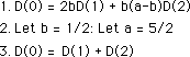
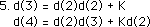
This means that even the Fibonacci series of Golden Mean fame is a special case of the D Series. If so, let us find the Limit of the ratio of its consecutive members. When ‘e’ and ‘f’ equal one as in the Fibonacci sequence then ‘b’ = 1/2 and ‘a’ = 5/2. As a check if one substitutes these two values into our general D Series, it reduces to the Fibonacci series. Shown here.
d(N) = 2(1/2)d(N-1) + (1/2)(5/2 - 1/2)d(N-2) = d(N-1) + d(N-2).
What is the Limit of the ratio of consecutive members of the Fibonacci sequence
Remember some basics.
Some simple algebra.
Hence the ratio of consecutive members of the Fibonacci series would be (√5 - 1)/2.
The Fibonacci series is a special case of the D Series for square roots. Indeed any 2nd order iterative equation that is based upon some function of the sum of its two previous elements is a member of the D Series set. As such they all possess a distinct and namable limit.
Now that we have examined some other features of the D Series, individual and universal, let us derive an even more general expression for the D Series. We will use a content-based approach to come upon this new expression.
For simplicity, let us begin with the same ‘seeds’ that we did before, i.e. 0 and 1.
Eq. 2 is the general expression for the D Series for square roots from Theorem 3.
With the two seeds from Eq. 1 we easily generate an expression for d(2).
Seeing that the coefficient for d(N-1) in the general expression is 2b, which is d(2), we rewrite the general expression with d(2) as coefficient instead.
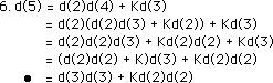
Using equation 4 we generate expressions for d(3) and d(4) above and d(5) below.
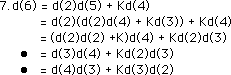
In a process, that we will repeat many times, we first expand the d(4) term in equation 6. We then multiply through by d(2). We then factor out the d(3) term. Inside the parentheses is d(3). The last equation reveals the transformed expression. It is an equation for d(5) where the coefficients are elements of the D series.
Using equation 4 we generate d(6). Using the same process as above, we first expand d(5). We then multiply through by d(2), and factor out d(4) from the first and third terms. Inside the parentheses is d(3). We rewrite the expression for d(6) in terms of members of the denominator series. Using the same process, we can generate a further reduction in a similar fashion.
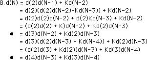
Let us apply this same process to Equation 4, the general expression for d(N). We first expand d(N-1) by the same Equation 4 that gave us d(N). We then multiply through by d(2), and factor out d(N-2) from the first and third terms. Inside the parentheses is d(3). We rewrite the expression for d(N) in terms of the reduced members of the D series. Using the same process, we can generate a further reduction in a similar fashion. We expand d(N-2), factor out d(N-3), replace what's inside the parenthesis by d(4), and then rewrite the reduced expression for d(N).
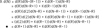
Finally we look at the most general expression. We start with coefficients in the same relationship that we observed before, which we will elucidate below. We expand d(N-R+1) by equation 4. We then multiply through by d(R), and then factor out d(N-R) from the first and third terms. Inside the parentheses is d(R+1). We then rewrite the expression for d(N) in terms of members of the D Series. Using the same process, we can generate a further reduction in a similar fashion.
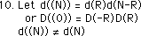
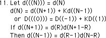
To clarify this general expression, we introduce another notational clarification. We let d((N)) equal a product of two members of the D Series, where the two numbers of the D series must add up to N. We are not talking about the actual value of the element of the D series; we are talking about its ordinal number in the series. d((N)) could equal the first element of the denominator series times the N-1 element in the series. It could also equal the product of the 2nd and N-2 element in the series. The first and second equations below are the same just written with a different notation. Let it be noted that d((N)) does not equal d(N).
Finally we let d(((N))) = d(N), just to clarify between the general expression above and the new notation. The triple parentheses just indicate a further layer of nested equations. We now rewrite d(N) or D(0) in terms of the new notation. We see that d(N) is the sum of a N+1 D Series product and a scaled N-1 D Series product.
There is one final condition. A N+1 denominator product, d((N+1)), could include d(2)d(N-1), d(3)d(N-2), etc. This is similar for a N-1 denominator product. However in the equation for d(N), the d((N+1)) and d((N-1)) products are linked. The terms of the d((N-1)) product must always be one less than the terms of the d((N+1)) product. In other words, if d((N+1)) = d(2)d(N-1), then d((N-1)) must equal d(1)d(N-2).
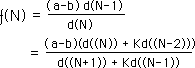
Let us reflect upon what we have just discovered. In examining the patterns of the D Series, we found an incredible underlying structure. At first glance each element of any D Series is formed by the sum of the two subsequent elements, each with its own coefficient. (When the coefficients are one, we have the Fibonacci Series, as a special case.) Upon closer look the coefficients become members of the D Series. Instead of the sum of the two subsequent elements, we instead have the sum of two products of earlier members of the series. This sum of products is tightly regulated. Once one of the members is known the others follow. Further it is possible that neither of the two preceding elements is included in this sum of products. Also the second of the two products is always scaled by a constant, K = b(a-b). Below are representations of our square root function in general terms.
These are not designed for simplicity but to illustrate the underlying complexity of the F&D series which determines square roots, whose patterns, in some ways, could be called the number itself. Hence each number has an incredibly complex, tightly defined structure, based upon the D Series, which is crystalline in its rigidity of form, but sparkles with the variety that it is able to express its individuality. Depending upon how you look at it, it will look differently and yet be the same once it manifests.
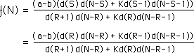
Here are two more representations of the F Series for square roots. The first acknowledges the independence of expression between d(N-1), which uses S as its variable, and d(N), which uses R as its variable. The second expression sets S=R. It illustrates the parallel expressions in the top and bottom. Bless Mother Nature in her complexity in the midst of her simplicity.
In this generalization of the Denominator Series, we see a type of power law in action. If we look at each member of the expression we see that as one side grows the other side falls and vice versa. We have a pile of equal numbers that represent clusters of events of the same magnitude. Each event can manifest in an infinite number of ways. Each number is a sum of products. The first element of each product would be the frequency of occurrence and the second would represent the magnitude of the events. As the frequency increased the size would shrink. Vice versa as the frequency shrank the magnitude of the events would grow. When the size would be at a maximum, the frequency would be at a minimum. When the size would be minimum then the frequency would be at a maximum. For instance, if each number were associated with earthquakes then as the frequency of earthquakes increased their magnitude would decrease. Vice versa as the frequency decreased the magnitude would increase. The overall pressure is the same. It can be diffused in many small earthquakes or in one large earthquake. The pressures of life build constantly. Either the tension can be diffused in many small explosions or in one big one. These examples are pure talk, potentially real or false but unsubstantiated.
Basically this section discovered the amazing self-reflective quality of our D Series for square roots. This expression of the D Series needs only one coefficient, the b(a-b) term. The first coefficient is replaced by one of the members of the D Series itself. Each element of the D Series can be generated by the sum of two distinct D Series products. One of these products is between two D Series elements, whose ordinal sum is one more than the ordinal number of the D element to be computed while the other product is based upon two elements of the D Series where the sum is one less than the D element to be computed.
Let us give an example of this internal symmetry of our D Series. The 16th element of all the infinite number of D Series is given by the sum of the product of the 10th and 7th element and the product of the 9th and 6th element times b(a-b). Or it could be the sum of the product of the 11th and 6th element and the product of the 10th and 5th element times b(a-b). Or it could be the sum of the product of the 9th and 8th element and the product of the 8th and 7th element times b(a-b). Or from the original D Series it could be the sum of the product of the 15th and 2nd element and the product of the 14th and 1st element times b(a-b). Because the 1st element equals one and the second equals 2b, we get our standard expression for the D Series. This internal symmetry is unique to the polarities of the D Series for square roots.